There’s a nice blog post from last year called Go smol or go home. If you’re training a large language model (LLM), you need to choose a balance between training compute, model size, and training tokens. The Chinchilla scaling laws tell you how these trade off against each other, and the post was a nice guide to the implications.
A new paper shows that the original Chinchilla scaling laws (from Hoffmann et al.) have a mistake in the key parameters. So below I’ve recalculated some scaling curves based on the corrected formulas.
Background
The Chinchilla neural scaling law1 gives a relationship between a model’s performance (loss), and the amount of training compute, training tokens and the number of parameters in the model. When people refer to “Chinchilla optimality”, they typically mean the point which minimizes training compute. I’ll refer to this as the Chinchilla point. However, in many situations this point is not what you want. Smaller models are more efficient at inference time, so if you’re doing a lot of inference, spending more compute at training time can reduce your overall compute budget. This is why models like Llama are trained far beyond the Chinchilla point. Microsoft’s Phi-3 models go in the same direction, to squeeze maximum performance into a model that can fit on a smartphone.
Revised Chinchilla formula
Here’s the change to the Chinchilla laws from the new paper:
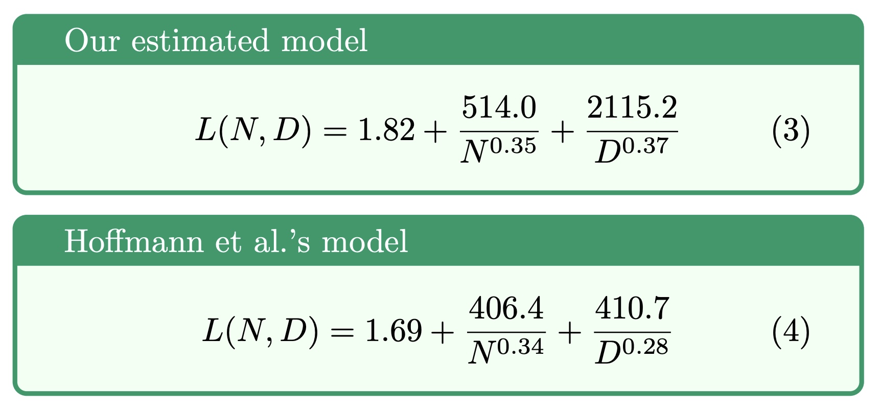
Results
Working things through as per this blog post, the revised results are below. Notably, the compute requirements come out higher at lower parameter counts.
| Parameter Count (1=Chinchilla optimal wrt training compute) | Compute | Token Requirement |
| 1x | 1x | 1x |
| 0.75 | 1.03 | 1.4 |
| 0.5 | 1.26 | 2.5 |
| 0.4 | 1.59 | 4 |
| 0.3 | 2.66 | 8.9 |
| 0.25 | 4.62 | 18.5 |
| 0.2 | 15.43 | 77.1 |
| 0.175 | 65.81 | 376.1 |
The way to read this table is that, for example, if you limit your model to 50% of the parameters of the Chinchilla point model, it will achieve the same loss with 26% more training compute and 2.5x the training tokens.
You can use this as a ready reckoner to understand a wide variety of models. A Chinchilla optimal model requires 15 – 25 tokens per parameter to train. Meta’s recent Llama3 70B model was trained with about 200 tokens per parameter, which is about 10x the Chinchilla point. Reading down the right column above, you can see that Llama 3 70B should therefore need about 3x the training compute, but only ~27% the parameters (implying inference is 3.7x cheaper), in order to achieve the same loss. Those numbers aren’t meant to be exact, but they should be close. Another way to think about it is that it should perform like a Chinchilla optimal model of about 260B params. That goes some way to explaining the high performance it achieves on benchmarks.
Microsoft’s Phi-3 model goes even further, training on 870 tokens per parameter, which is ~45x the Chinchilla point. Llama 3 8B goes further still, at 75x the tokens per parameter. These models require about 10x-15x the training compute, but only ~20% of the parameters (and thus get 5x inference performance) of the equivalent Chinchilla optimal model.
The scaling laws suggest you can’t go much further than that, as you start to hit an asymptote as the parameter count drops below 20%2. It will be interesting to see if this holds up, or if there are tricks that let you do better. Related work by Meta found that there’s a limit of 2 bits per parameter for what an LLM can store, which would imply a hard limit on the loss. The technical report for Phi-3 3.8B also reads like they’re bumping up against the limits of what can be achieved within that parameter budget. So it seems like this limit might hold, short of an architectural change to the models.
Undertrained models
People don’t talk about this so much, but you can also go in the other direction, i.e. train models with more parameters than Chinchilla optimal:
| Parameter Count (1=Chinchilla optimal wrt training compute) | Compute | Token Requirement |
| 1 | 1 | 1 |
| 2 | 1.15 | 0.57 |
| 3 | 1.37 | 0.46 |
| 4 | 1.59 | 0.4 |
| 5 | 1.81 | 0.36 |
| 10 | 2.88 | 0.29 |
| 100 | 19.07 | 0.19 |
| 1000 | 161.57 | 0.16 |
Increasing the parameter count past the Chinchilla point gives a model that’s more RAM hungry, more expensive to train and more expensive at inference time. However, it does reduce training token requirements, in the limit as much as 6x (i.e down to about 16% of the Chinchilla point). You might want to do this if you had a small model in a data poor regime, and there was no way to spend the extra compute more productively (e.g on synthetic data). This might apply in some robotics or medical problems perhaps.
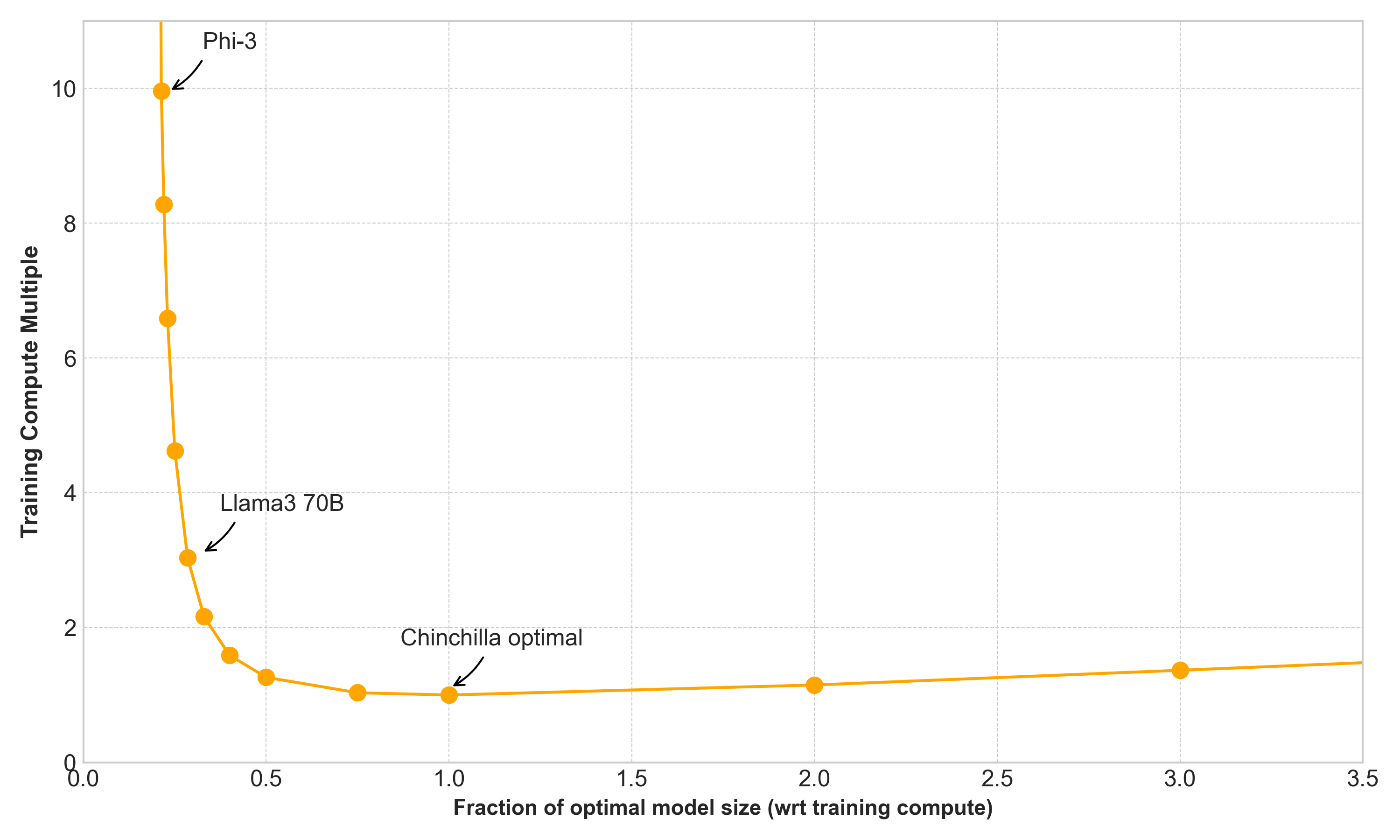
Graphs
I’m not as talented a graph maker as the author of the original post, but here’s some plots of the curves.
Firstly, compute requirement as a function of model size:
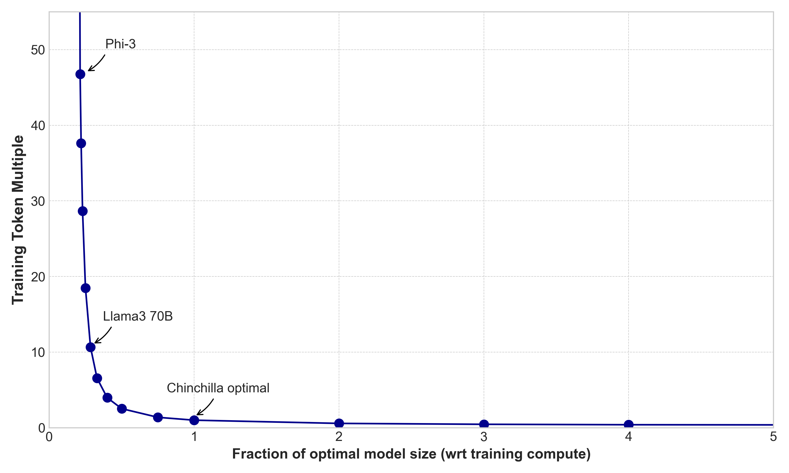
Secondly, training data requirement as a function of model size:
Footnotes
- It’s widely referred to as a scaling law, though it’s worth remembering that it’s just an empirical fit to data. There’s no guarantee it holds everywhere and forever. ↩︎
- For example, to get a model down to 15% of the parameters, the formula suggests you need almost 600,000x the compute and 4,000,000x the tokens. ↩︎
Comments are closed.